🗄️
Chapter 1.1 — Overview of Databases
🗄️ CHAPTER 1.1 — OVERVIEW OF DATABASES MIND MAP
DBMS vs File System → Less redundancy, better integrity, concurrent access, security, data independence
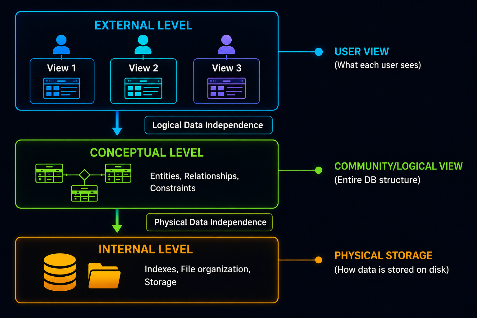
ANSI-SPARC → External (user views) → Conceptual (whole DB structure) → Internal (physical storage)
Data Independence → Logical (conceptual changes don't break apps) vs Physical (storage changes don't break conceptual)
Schema vs Instance → Schema = structure/blueprint, Instance = actual data right now
Keys → Super → Candidate (minimal) → Primary (chosen) + Alternate (not chosen) + Foreign (references)
Integrity → Entity (PK not null) + Referential (FK matches PK or null)
DBA → Schema, Security, Performance, Availability
1. DBMS — Basic Concepts, Components & Architecture
📖 Database: An organized collection of related data stored electronically.
📖 DBMS (Database Management System): Software that allows users to define, create, maintain, and control access to a database.
DBMS vs File System:
| Feature | File System | DBMS |
|---|
| Data Redundancy | High (same data repeated in multiple files) | Minimized (centralized data) |
| Data Integrity | Hard to enforce | Enforced via constraints |
| Concurrent Access | Difficult, prone to conflicts | Managed via locking/transactions |
| Security | File-level only | Fine-grained (table/row/column level) |
| Data Independence | None — programs depend on file structure | Yes — programs shielded from storage details |
Components of a DBMS Environment:
| Component | Role |
|---|
| Hardware | Physical devices — servers, storage disks |
| Software | The DBMS itself, OS, and application programs |
| Data | The actual facts stored (the most important asset) |
| Procedures | Instructions/rules for using and administering the database |
| Users | DBA, application programmers, end users |
Types of DBMS Users:
1. Database Administrator (DBA) — manages the entire database system
2. Application Programmers — write programs that interact with the database via APIs
3. Sophisticated Users — interact using query languages directly (analysts)
4. Naive/End Users — interact via pre-built forms/applications (e.g. ATM users)
💡 Exam Tip: "Data Redundancy" and "Data Inconsistency" are commonly confused — redundancy is the CAUSE (same data stored multiple times), inconsistency is the EFFECT (copies going out of sync when one is updated but not others).
2. ANSI-SPARC Three-Level Architecture & Data Independence
📖 Why layers? The ANSI-SPARC architecture separates HOW data is physically stored from HOW users view it — different users can see different views of the same underlying data.
🏗️ ANSI-SPARC Three-Level Architecture
| Level | Describes | Example |
|---|
| External (View Level) | What each individual user sees — a customized subset | A student sees only their own grades, not others' |
| Conceptual (Logical Level) | The complete logical structure of the whole database — entities, relationships, constraints — for the entire community of users | All tables, their columns, and relationships |
| Internal (Physical Level) | How data is actually stored on disk — file structures, indexes, access paths | B-tree index files, block sizes |
Data Independence:
Logical Data Independence: Ability to change the conceptual schema (e.g. add a new table/column) WITHOUT changing external schemas or application programs.
Physical Data Independence: Ability to change the internal schema (e.g. change file storage or indexing) WITHOUT changing the conceptual schema.
💡 Worked Example — Logical Data Independence:
A college database has a STUDENT table (RollNo, Name, Branch). The admin adds a new column "Email" to support a notification feature.
→ Existing application programs that only ever used RollNo, Name, Branch continue to work UNCHANGED — they simply don't reference the new Email column. The conceptual schema changed, but external views/programs didn't need modification.
💡 Worked Example — Physical Data Independence:
The DBA decides to switch the STUDENT table's storage from a simple heap file to a B-tree indexed file for faster lookups.
→ All existing queries (SELECT * FROM STUDENT WHERE RollNo=101) still return the SAME results, written the SAME way — the conceptual/logical view of the table never changed, only the underlying physical storage mechanism did.
💡 Exam Tip: Logical data independence is HARDER to achieve than physical — because changing the logical structure (like removing a table) is far more likely to break existing application code than changing storage details underneath.
3. Schema vs Instance & Types of Database Keys
📖 Schema: The overall STRUCTURE/design of the database — table names, column names, data types, and constraints. Rarely changes.
📖 Instance: The actual DATA stored in the database at a particular moment in time. Changes constantly (every INSERT/UPDATE/DELETE).
💡 Analogy: Schema = the blank form/template (fields: Name, Roll No, Marks). Instance = the form filled out with actual student data right now.
Types of Database Keys:
| Key Type | Definition |
|---|
| Super Key | Any set of one or more attributes that can uniquely identify a tuple (row) |
| Candidate Key | A MINIMAL super key — no attribute can be removed without losing uniqueness |
| Primary Key | The candidate key CHOSEN to uniquely identify rows; cannot be NULL |
| Alternate Key | Candidate key(s) NOT chosen as the primary key |
| Foreign Key | An attribute in one table that refers to the Primary Key of another (or same) table |
| Composite Key | A key made up of TWO or more attributes together (none alone is unique) |
💡 Worked Example — STUDENT(RollNo, Email, Aadhaar, Name):
• RollNo, Email, and Aadhaar are each individually unique → each is a Candidate Key
• {RollNo, Email, Aadhaar} together is a Super Key (not minimal though)
• Say RollNo is chosen as Primary Key → Email and Aadhaar become Alternate Keys
💡 Exam Tip: "Every Candidate Key is a Super Key, but not every Super Key is a Candidate Key" — because a Super Key can have extra unnecessary attributes; a Candidate Key cannot (it's minimal).
4. Entity Integrity & Referential Integrity Constraints
📖 Integrity Constraints: Rules that ensure the accuracy and consistency of data in the database.
A. Entity Integrity Constraint:
Rule: No attribute of a Primary Key can be NULL.
Why: The primary key's job is to uniquely identify each row — a NULL value can't uniquely identify anything.
-- VIOLATES Entity Integrity (RollNo is Primary Key)
INSERT INTO Student (RollNo, Name) VALUES (NULL, 'Ankush');
-- ❌ Rejected by DBMS
B. Referential Integrity Constraint:
Rule: A Foreign Key value must either MATCH a Primary Key value in the referenced (parent) table, OR be entirely NULL.
Why: Prevents "orphan" records that point to non-existent parent rows.
-- Enrollment(StudentID references Student.RollNo)
-- VIOLATES Referential Integrity:
INSERT INTO Enrollment (StudentID, Course) VALUES (999, 'DBMS');
-- ❌ Rejected if RollNo 999 doesn't exist in Student table
| Constraint | Applies To | Rule |
|---|
| Entity Integrity | Primary Key | Cannot be NULL |
| Referential Integrity | Foreign Key | Must match existing PK value, or be NULL |
💡 Exam Tip: Referential integrity violations commonly happen on DELETE — if you try to delete a parent row that child rows still reference, the DBMS blocks it (or cascades, depending on the ON DELETE rule set).
5. Database Administrator (DBA) — Roles & Responsibilities
📖 DBA: The person (or team) responsible for the overall control, management, and security of a database system.
| Responsibility | What It Involves |
|---|
| Schema Definition | Creating the original database schema by writing DDL statements |
| Storage & Access Definition | Deciding storage structure and access methods for performance |
| Access Authorization | Granting/revoking different levels of access permission to users |
| Routine Maintenance | Backups, monitoring disk usage, ensuring smooth operation |
| Integrity Constraint Specification | Defining rules the data must satisfy (keys, checks) |
| Liaising with Users | Gathering requirements, resolving data-related issues |
In short, the DBA controls 4 major things:
1. Schema — the design
2. Security — who can access what
3. Performance — indexing, tuning
4. Availability — backup and recovery
💡 Exam Tip: Don't confuse DBA with Database Designer — the Designer decides WHAT the schema should look like (during design phase); the DBA maintains and secures it once it's live (during operation phase). In small teams, one person may do both.
📊
Chapter 1.2 — Data Models
📊 CHAPTER 1.2 — DATA MODELS MIND MAP
3 Models → Hierarchical (tree, 1 parent) → Network (graph, multi-parent) → Relational (tables, declarative)
ER Diagram → Entity (rectangle), Attribute (ellipse), Relationship (diamond)
Attributes → Simple, Composite, Derived, Multivalued, Key
EER → Specialization (top-down) / Generalization (bottom-up) = ISA hierarchy; Aggregation = relationship as entity
Mapping Constraints → Cardinality (1:1, 1:N, M:N) + Participation (Total/Partial)
ER→Relational → Entity=table, 1:N=FK on many side, M:N=new junction table
1. Relational, Network & Hierarchical Data Models
📖 Data Model: A conceptual way of organizing data elements and specifying how they relate to one another.
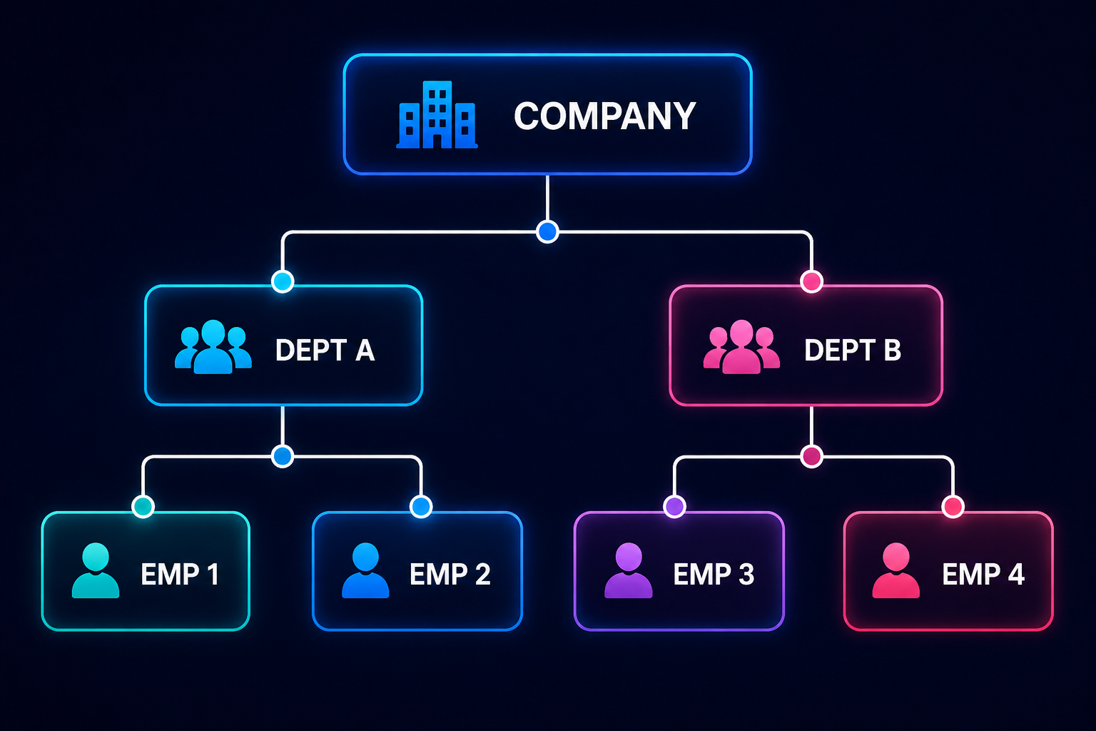
A. Hierarchical Model — Tree Structure:
B. Network Model — Graph Structure:
Similar to hierarchical, but a child (member) CAN have MULTIPLE parents (owners) — represented as a graph, not strictly a tree. Uses "owner-member" set relationships (CODASYL model).
C. Relational Model — Tables:
Data organized into TABLES (relations) made of rows (tuples) and columns (attributes). Relationships are represented using Foreign Keys, not physical pointers. This is the model almost all modern DBMS (MySQL, Oracle, PostgreSQL) use.
| Feature | Hierarchical | Network | Relational |
|---|
| Structure | Tree | Graph | Table (rows/columns) |
| Parent-Child | 1 parent only | Multiple parents allowed | No pointers — Foreign Keys |
| Flexibility | Low, rigid | Medium, complex navigation | High, query-based (SQL) |
| Ease of Use | Hard — needs traversal knowledge | Hard — complex pointers | Easy — declarative queries |
💡 Exam Tip: Hierarchical and Network models are "navigational" (you must know the path/pointers to get data); the Relational model is "declarative" (you just say WHAT you want via SQL, not HOW to get it) — this is the single biggest advantage that made relational databases dominant.
2. ER Diagrams — Entity-Relationship Modeling
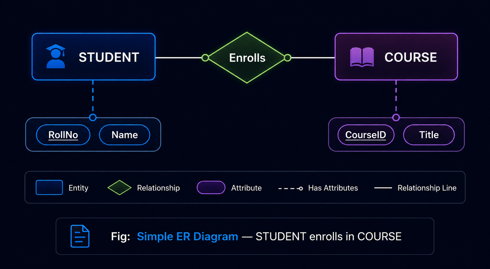
📖 ER Model: A high-level conceptual data model that describes data as Entities, Attributes, and Relationships — used to visually design a database before creating tables.
| Symbol | Represents | Example |
|---|
| ▭ Rectangle | Entity — a real-world object/concept | Student, Course |
| ○ Ellipse | Attribute — a property of an entity | Name, RollNo |
| ◇ Diamond | Relationship — association between entities | Enrolls, Teaches |
| — Line | Connects entity to attribute/relationship | — |
Types of Attributes:
| Attribute Type | Meaning | Example |
|---|
| Simple | Cannot be divided further | Age |
| Composite | Can be split into sub-parts | Address → Street, City, Pincode |
| Derived | Calculated from another attribute | Age (derived from Date of Birth) |
| Multivalued | Can hold more than one value | PhoneNumbers (a person may have several) |
| Key Attribute | Uniquely identifies the entity (underlined in diagrams) | RollNo |
💡 Exam Tip: A "weak entity" (drawn with a double rectangle) cannot exist without a related "strong entity" — e.g. an Employee's Dependent has no meaning without the Employee. Its key is called a "partial key" (dashed underline).
3. EER Diagrams — Extended ER Model
📖 EER Model: An extension of the basic ER model that adds support for modeling more complex real-world scenarios — Generalization, Specialization, and Aggregation.
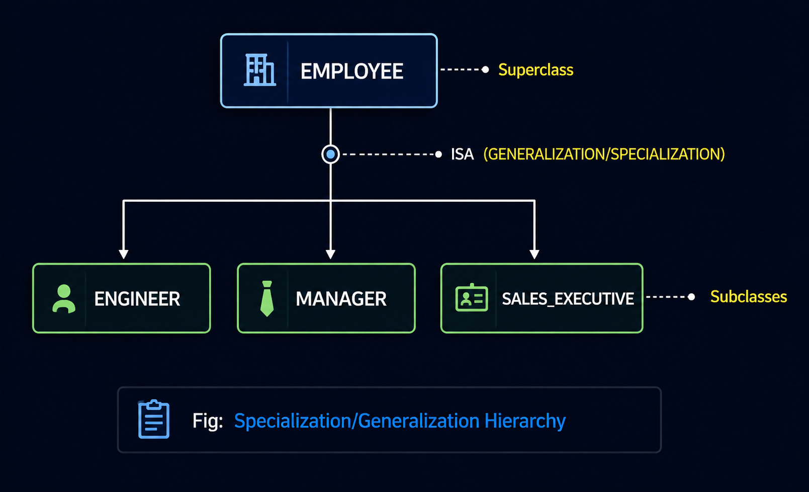
A. Specialization (Top-Down):
Starts with a general Superclass entity and divides it into more specific Subclass entities based on distinguishing features.
Example: EMPLOYEE (superclass) specialized into ENGINEER, MANAGER, SALESPERSON (subclasses)
B. Generalization (Bottom-Up):
The reverse process — starts with multiple specific entities and combines their common features into one general Superclass.
Example: CAR and TRUCK generalized into VEHICLE
🧠 Specialization / Generalization Hierarchy
C. Aggregation:
📖 Aggregation: Treats a RELATIONSHIP itself as a higher-level entity, so it can participate in further relationships with other entities. Used when a relationship needs its own relationship.
| Concept | Direction | Purpose |
|---|
| Specialization | Top-down (general → specific) | Divide a general entity into meaningful subtypes |
| Generalization | Bottom-up (specific → general) | Combine common features of similar entities |
| Aggregation | Relationship → treated as Entity | Allow a relationship to have its own relationships |
💡 Exam Tip: Specialization and Generalization describe the SAME "ISA" hierarchy structure — they only differ in the DIRECTION you designed it (top-down vs bottom-up). The resulting diagram looks identical either way.
4. Mapping Constraints & Relationships in ER Modeling
📖 Mapping Cardinality: Specifies HOW MANY instances of one entity can be associated with how many instances of another entity via a relationship.
| Cardinality | Meaning | Example |
|---|
| One-to-One (1:1) | One entity A relates to exactly one entity B, and vice versa | Person ↔ Passport |
| One-to-Many (1:N) | One entity A can relate to MANY entity B, but each B relates to only one A | Department → Employees |
| Many-to-One (N:1) | Same as 1:N, viewed from the other side | Employees → Department |
| Many-to-Many (M:N) | Many entities A relate to many entities B | Students ↔ Courses |
Participation Constraints:
Total Participation (double line in ER diagram): EVERY instance of the entity MUST participate in the relationship.
Example: every Employee MUST work in some Department.
Partial Participation (single line): Some instances may NOT participate.
Example: not every Employee MUST manage a project.
💡 Combining Both: A relationship can have BOTH cardinality AND participation specified together — e.g. "Every Employee (total participation) works in exactly one Department (1:N cardinality from Department's side)."
Min-Max Notation:
📖 Min-Max Constraint: A more PRECISE way of writing both cardinality AND participation together as a single pair (min, max) attached to each entity's side of a relationship — instead of stating them as two separate constraints.
min = the MINIMUM number of relationship instances an entity occurrence must participate in (0 = optional/partial, 1 or more = mandatory/total)
max = the MAXIMUM number of relationship instances an entity occurrence can participate in (1 = single, N = many)
DEPARTMENT (0,N)◇──WORKS_IN──◇(1,1) EMPLOYEE
Fig: Min-Max Notation for a 1:N Relationship
💡 Worked Example — One-to-Many: DEPARTMENT — EMPLOYEE:
Employee side: (1,1) → min=1 (every Employee MUST work in a department — total participation) and max=1 (each Employee works in exactly ONE department — the "many-to-ONE" side).
Department side: (0,N) → min=0 (a Department can exist even with zero employees currently assigned — partial participation) and max=N (a Department can have MANY employees).
This single (min,max) pair notation captures BOTH the cardinality (1:N) AND participation (total/partial) that would otherwise need two separate constraints to express.
💡 Exam Tip: min=0 always means Partial participation; min≥1 always means Total participation. max=1 means "one" side of the relationship; max=N means "many" side. Reading a (min,max) pair, always state BOTH what it means for participation AND for cardinality.
💡 Exam Tip: Cardinality answers "HOW MANY", Participation answers "IS IT MANDATORY". These are two separate, independent constraints often tested together in one diagram-drawing question.
5. Converting ER/EER Models to Relational Schema
📖 Why convert? ER diagrams are a conceptual DESIGN tool — but a DBMS stores data in TABLES. These mapping rules convert the diagram into actual relational tables.
| ER Construct | Maps To |
|---|
| Strong Entity | A separate table; key attribute → Primary Key |
| Weak Entity | A table whose Primary Key = its partial key + owner entity's Primary Key (as Foreign Key) |
| 1:1 Relationship | Foreign Key placed in EITHER table (usually the one with total participation) |
| 1:N Relationship | Foreign Key placed on the "Many" side table |
| M:N Relationship | A NEW separate table created, holding Foreign Keys from BOTH entities |
| Multivalued Attribute | A separate table, with Foreign Key referring back to the owning entity |
💡 Worked Example — STUDENT enrolls in COURSE (M:N):
STUDENT(RollNo, Name)
COURSE(CourseID, Title)
ENROLLS(RollNo, CourseID) — new table, both are Foreign Keys, together form the Primary Key
💡 Worked Example — DEPARTMENT has EMPLOYEES (1:N):
DEPARTMENT(DeptID, DeptName)
EMPLOYEE(EmpID, Name, DeptID) — DeptID is Foreign Key referencing DEPARTMENT (no new table needed)
💡 Exam Tip: M:N relationships ALWAYS need a new junction/bridge table — this is the single most commonly tested mapping rule, since 1:1 and 1:N can be handled with just a Foreign Key column.
🧮
Chapter 1.3 — Relational Algebra and Relational Calculus
🧮 CHAPTER 1.3 — RELATIONAL ALGEBRA & CALCULUS MIND MAP
Algebra (Procedural) → σ Selection(rows), π Projection(columns), ∪ Union, − Difference, × Product, ρ Rename
Joins → Theta(any op) → Equijoin(only =) → Natural(= + drop duplicate column)
Division (÷) → Find rows related to ALL rows of another relation
TRC → { t | P(t) } — variable = whole tuple, uses t.attribute
DRC → { <x,y,z> | P(x,y,z) } — variable per domain/column value
Algebra vs Calculus → Procedural(HOW) vs Non-procedural(WHAT) — both "Relationally Complete"
1. Relational Algebra — Basic Operations
📖 Relational Algebra: A PROCEDURAL query language — a set of operations that take one or two relations (tables) as input and produce a new relation as output. It describes HOW to get the result, step by step.
| Operation | Symbol | Purpose |
|---|
| Selection | σ (sigma) | Selects ROWS matching a condition |
| Projection | π (pi) | Selects specific COLUMNS |
| Union | ∪ | Combines rows from two relations (removes duplicates) |
| Set Difference | − | Rows in R1 but NOT in R2 |
| Cartesian Product | × | Every row of R1 paired with every row of R2 |
| Rename | ρ (rho) | Renames a relation or its attributes |
Worked Examples — STUDENT(RollNo, Name, Branch, Marks):
-- SELECTION: rows where Branch = 'CSE'
σ(Branch='CSE') (STUDENT)
-- PROJECTION: only Name and Marks columns
π(Name, Marks) (STUDENT)
-- COMBINED: Names of CSE students
π(Name) (σ(Branch='CSE') (STUDENT))
-- UNION: students who are in CSE_LIST or ECE_LIST
CSE_LIST ∪ ECE_LIST
-- SET DIFFERENCE: students in ALL_STUDENTS but not in PASSED
ALL_STUDENTS − PASSED
Rules for Union & Set Difference (Union-Compatibility):
Both relations must have the SAME number of attributes, and corresponding attributes must have the SAME domain (data type).
📖 Why is Union Compatibility Required?
UNION (∪), INTERSECTION (∩), and DIFFERENCE (−) all work by comparing and combining TUPLES (rows) between two relations, position by position. This ONLY makes logical sense if:
1. Both relations have the same NUMBER of columns — otherwise there's no consistent way to align/compare tuples.
2. Corresponding columns share the same DOMAIN — otherwise you could get nonsensical results (e.g. comparing a Name column with a Salary column just because they're both in position 2).
💡 Why It Breaks Without Compatibility:
CSE_STUDENTS(RollNo, Name) has 2 columns. FACULTY(EmpID, Name, Dept) has 3 columns.
CSE_STUDENTS ∪ FACULTY → ❌ INVALID — different number of attributes, so the DBMS has no way to decide which columns correspond to which, making the union meaningless.
💡 Exam Tip: Selection (σ) filters ROWS (like SQL's WHERE clause); Projection (π) filters COLUMNS (like SQL's SELECT column list). This σ vs π mix-up is the #1 mistake students make.
2. Relational Algebra — Join & Other Derived Operators
📖 Derived Operators: Operations that CAN technically be built from the basic 6 operators, but are so commonly needed they get their own symbol for convenience.
| Operation | Symbol | Purpose |
|---|
| Intersection | ∩ | Rows common to BOTH relations |
| Theta Join | ⋈θ | Cartesian Product + condition (θ can be any comparison: =, <, >) |
| Equijoin | ⋈ | Theta Join where condition uses ONLY "=" |
| Natural Join | ⋈ | Equijoin on common attribute name(s), duplicate column automatically removed |
| Division | ÷ | Finds rows in R1 related to ALL rows in R2 |
Worked Example — Natural Join:
STUDENT(RollNo, Name, DeptID)
DEPARTMENT(DeptID, DeptName)
-- Natural Join: combines on common attribute "DeptID"
STUDENT ⋈ DEPARTMENT
-- Result: RollNo, Name, DeptID, DeptName
-- (DeptID appears only ONCE — duplicates auto-removed)
Worked Example — Division (÷):
💡 Classic use case: "Find students who have enrolled in ALL courses offered."
ENROLLS(RollNo, CourseID) ÷ COURSE(CourseID)
→ Returns only RollNo values that appear against EVERY CourseID in the COURSE table.
| Join Type | Key Difference |
|---|
| Theta Join | Any comparison operator (=, <, >, ≠...) |
| Equijoin | Only "=" comparison; duplicate columns still present |
| Natural Join | Equijoin + automatically drops duplicate column |
💡 Exam Tip: Natural Join is just Equijoin with the extra step of removing the duplicate attribute column — this exact distinction is a very common 2-mark "differentiate" question.
3. Tuple Relational Calculus (TRC)
📖 Relational Calculus: A NON-PROCEDURAL (declarative) query language — you describe WHAT result you want, not HOW to compute it (unlike Relational Algebra).
📖 TRC: Uses TUPLE variables that range over rows of a relation.
General Syntax:
{ t | P(t) }
Read as: "the set of all tuples t such that predicate P(t) is true"
Worked Example — STUDENT(RollNo, Name, Branch, Marks):
-- Find all students in 'CSE' branch:
{ t | t ∈ STUDENT AND t.Branch = 'CSE' }
-- Find names of students with Marks > 80:
{ t.Name | t ∈ STUDENT AND t.Marks > 80 }
Quantifiers Used in TRC:
| Quantifier | Symbol | Meaning |
|---|
| Existential | ∃ (there exists) | At least ONE tuple satisfies the condition |
| Universal | ∀ (for all) | ALL tuples must satisfy the condition |
💡 With Existential Quantifier:
"Find names of students who have enrolled in at least one course":
{ t.Name | t ∈ STUDENT AND ∃ e ∈ ENROLLS (e.RollNo = t.RollNo) }
💡 Exam Tip: TRC variable "t" represents a WHOLE ROW (tuple) — you access individual columns using dot notation like t.Name, t.Marks. This is the key structural difference from Domain Calculus (next topic).
4. Domain Relational Calculus (DRC)
📖 DRC: Similar to TRC, but instead of tuple variables, DRC uses DOMAIN variables — one variable per individual COLUMN/attribute value, not the whole row.
General Syntax:
{ <x₁, x₂, ..., xₙ> | P(x₁, x₂, ..., xₙ) }
Read as: "the set of all <x₁...xₙ> tuples such that predicate P is true"
Worked Example — STUDENT(RollNo, Name, Branch, Marks):
-- Find all students in 'CSE' branch:
{ | ∈ STUDENT AND b = 'CSE' }
-- Find names of students with Marks > 80:
{ n | ∈ STUDENT AND m > 80 }
| Feature | TRC | DRC |
|---|
| Variable represents | An entire TUPLE (row) | A single DOMAIN value (column) |
| Access syntax | t.attribute (dot notation) | Separate variable per attribute |
| Used by | QUEL language (historical) | QBE — Query By Example |
💡 Exam Tip: Easiest way to remember: TRC variable = ONE row, DRC variables = ONE value each (one per column). If a question shows angle-bracket <x,y,z> notation with separate variables, that's DRC; if it shows t.column dot-notation, that's TRC.
5. Relational Algebra vs Relational Calculus
📖 Core Difference: Algebra is PROCEDURAL (specifies the sequence of operations/steps); Calculus is NON-PROCEDURAL (specifies only the desired result, DBMS figures out how).
| Feature | Relational Algebra | Relational Calculus |
|---|
| Nature | Procedural (HOW) | Non-procedural / Declarative (WHAT) |
| Approach | Step-by-step operations (σ, π, ⋈...) | Predicate/condition-based (logic formula) |
| Ease of Use | Requires knowing operation ORDER | Just describe the condition — order-free |
| Types | Single language | TRC (tuple-based) and DRC (domain-based) |
✅ Computational Equivalence — "Relationally Complete":
Relational Algebra and Relational Calculus (both TRC and DRC, when restricted to "safe" expressions) are PROVABLY EQUIVALENT in computational power — anything expressible in one CAN be expressed in the other. This equivalence is called being "Relationally Complete."
💡 Same Query, Both Ways — "Names of CSE students":
Algebra: π(Name) (σ(Branch='CSE') (STUDENT))
TRC: { t.Name | t ∈ STUDENT AND t.Branch = 'CSE' }
💡 Exam Tip: SQL itself is based on BOTH — its structure (SELECT-FROM-WHERE) resembles calculus (declarative), while its execution internally uses algebra-like operations. "Relationally complete" is the exact term examiners look for in this comparison question.
⚡
Ready for Exam?
Sab padh liya? Ab Quick Revision karo — key points aur formulas ek jagah!
Quick Revision Karo →
⚡
Quick Revision — Last Minute Exam Prep!
📌 How to Use: Read this 5-10 minutes before exam. Contains all important points in condensed form. Focus on tables, comparisons, and key formulas!
🗄️ Chapter 1.1 — Overview of Databases
📖 DBMS vs File System:
Less redundancy, better integrity, easier concurrent access, fine-grained security, data independence.
🔑 3 Levels (ANSI-SPARC):
External → individual user views
Conceptual → whole logical DB structure
Internal → physical storage/indexes
Data Independence:
Logical → conceptual change doesn't break external views
Physical → internal change doesn't break conceptual level
KEYS HIERARCHY:
Super Key → Candidate Key (minimal)
→ Primary Key (chosen one)
→ Alternate Key (not chosen)
→ Foreign Key (references another PK)
Quick Recall: every Candidate Key IS a Super Key, but not vice versa.
⚠️ Integrity Rules:
Entity Integrity → Primary Key can NEVER be NULL
Referential Integrity → Foreign Key must MATCH an existing PK, or be NULL
✅ DBA's 4 Jobs: Schema, Security, Performance, Availability (backup/recovery).
| Topic | Key Fact | Trick |
|---|
| ANSI-SPARC | External → Conceptual → Internal | Logical Independence > Physical (harder) |
| Schema vs Instance | Structure vs actual data now | Schema rarely changes |
| Keys | Super ⊇ Candidate ⊇ Primary | Candidate = minimal Super |
| Entity Integrity | PK ≠ NULL | Applies to Primary Key only |
| Referential Integrity | FK = existing PK or NULL | Prevents orphan rows |
📊 Chapter 1.2 — Data Models
📖 3 Data Models:
Hierarchical (tree, 1 parent only) → Network (graph, multi-parent, CODASYL) → Relational (tables, declarative SQL — modern standard).
🔑 ER Diagram Symbols:
▭ Rectangle → Entity
○ Ellipse → Attribute
◇ Diamond → Relationship
Attribute types: Simple, Composite, Derived, Multivalued, Key
EER CONCEPTS:
Specialization → top-down (general → specific)
Generalization → bottom-up (specific → general)
Aggregation → relationship treated as an entity
Quick Recall: Both Spec/Gen produce the SAME "ISA" hierarchy diagram — only direction of design differs.
✅ Mapping Constraints:
Cardinality (1:1, 1:N, M:N) = HOW MANY
Participation (Total/Partial) = IS IT MANDATORY
💡 ER → Relational Quick Recall:
1:N → Foreign Key on the "Many" side (no new table)
M:N → NEW junction table with both Foreign Keys
Example: ENROLLS(RollNo, CourseID) — both FKs, together = PK
| Topic | Key Fact | Trick |
|---|
| Data Models | Hierarchical→Network→Relational | Relational = declarative (SQL) |
| ER Symbols | Rect=Entity, Ellipse=Attr, Diamond=Rel | Weak entity = double rectangle |
| Specialization/Generalization | Top-down / Bottom-up | Same ISA hierarchy result |
| Cardinality | 1:1, 1:N, M:N | M:N always needs junction table |
🧮 Chapter 1.3 — Relational Algebra & Calculus
📖 Basic Algebra Operators:
σ Selection (rows) | π Projection (columns) | ∪ Union | − Difference | × Cartesian Product | ρ Rename
🔑 Quick Example Recall:
Names of CSE students:
π(Name) (σ(Branch='CSE') (STUDENT))
Trick: σ = WHERE clause (rows), π = SELECT column-list (columns) — most common mix-up.
JOIN TYPES:
Theta Join → any comparison operator
Equijoin → only "=", duplicate columns remain
Natural Join → Equijoin + drops duplicate column
Division (÷) → rows related to ALL rows of another relation
✅ TRC vs DRC:
TRC → { t | P(t) }, variable = whole tuple, uses t.attribute
DRC → { <x,y,z> | P(x,y,z) }, variable per column value
💡 Algebra vs Calculus — Same Query:
Algebra: π(Name) (σ(Branch='CSE') (STUDENT))
TRC: { t.Name | t ∈ STUDENT AND t.Branch = 'CSE' }
Both are "Relationally Complete" — provably equal computational power.
| Topic | Key Fact | Trick |
|---|
| Selection vs Projection | σ=rows, π=columns | σ→WHERE, π→SELECT list |
| Natural Join | Equijoin + remove duplicate col | Common attribute auto-matched |
| TRC | { t | P(t) } | t.attribute dot notation |
| DRC | { <x,y> | P(x,y) } | One variable per column |
| Algebra vs Calculus | Procedural vs Non-procedural | Both Relationally Complete |
⚠️ Common Exam Mistakes
❌ Confusing Super Key with Candidate Key — every Candidate Key is a Super Key, not the reverse
❌ Writing Entity Integrity rule for Foreign Key (it's for Primary Key — FK gets Referential Integrity)
❌ Mixing up σ (Selection = rows) with π (Projection = columns)
❌ Forgetting Natural Join removes the duplicate common column, unlike Equijoin
❌ Writing DRC with dot-notation (t.attribute) — that's TRC syntax, not DRC
❌ Forgetting M:N relationships need a NEW junction table, not just a Foreign Key column
❌ Mixing up Logical vs Physical Data Independence direction
✅ Pre-Exam Checklist
☑ DBMS vs File System advantages
☑ ANSI-SPARC 3 levels + Logical/Physical Data Independence
☑ Schema vs Instance distinction
☑ All key types — Super, Candidate, Primary, Alternate, Foreign, Composite
☑ Entity Integrity vs Referential Integrity
☑ DBA roles and responsibilities
☑ Hierarchical vs Network vs Relational models
☑ ER diagram symbols + attribute types
☑ EER — Specialization, Generalization, Aggregation
☑ Cardinality + Participation constraints
☑ ER-to-Relational mapping rules (especially M:N)
☑ Relational Algebra — all 6 basic operators
☑ Join types — Theta, Equijoin, Natural Join, Division
☑ TRC and DRC syntax + worked examples
☑ Relational Algebra vs Calculus — "Relationally Complete"
🎯 Exam Strategy
2 Mark Questions:
• Direct definition + 1 example. Time: 3-4 minutes.
• "Differentiate" → always draw a 2-column table.
5 Mark Questions:
• Definition + Diagram + Relational Algebra/Calculus expression. Time: 7-8 minutes.
• ER diagram questions — always label cardinality and participation clearly.
• Relational Algebra queries — write the expression AND explain each operator used.
Marks-saving tip:
Even if a full query expression isn't complete, writing the correct operators/symbols and the general structure earns partial marks!
🌟 All the Best!
DBMS Unit 1 is concept + diagram heavy — ER diagrams, key types, aur relational algebra expressions practice karo by hand. Tables aur symbol meanings yaad karo, aur tu ready hai! 💪🗄️
📄
Previous Year Questions
📌 Source: Mid Semester Test-1 (MST-1), Academic Year 2025-2026 — Unit 1 only. Maximum Marks: 20, Time: 1 Hour.
Section A (5 × 2 = 10 marks)
2M
MST-1
Differentiate between logical and physical data independence with an example.
▼
Logical Data Independence: Ability to change the conceptual schema without affecting external views/applications.
Example: Adding an "Email" column to STUDENT table — existing programs that don't use Email keep working unchanged.
Physical Data Independence: Ability to change the internal (storage) schema without affecting the conceptual schema.
Example: Switching STUDENT table's storage to a B-tree index — queries return the same results, written the same way.
Logical independence is harder to achieve than physical. Full explanation in Chapter 1.1, Section 2.
2M
MST-1
Articulate two critical responsibilities of a DBA and their importance in managing a database system.
▼
Any two of the following, with importance:
1. Schema Definition: The DBA creates and maintains the database structure via DDL — important because a well-designed schema prevents redundancy and ensures data integrity from the start.
2. Access Authorization: The DBA grants/revokes user permissions — important for data SECURITY, ensuring only authorized users can view/modify sensitive data.
(Other valid answers: Routine Maintenance/backups, Integrity Constraint Specification — see Chapter 1.1, Section 5 for the full list of 6.)
2M
MST-1
What is union compatibility? Why do the UNION, INTERSECTION, and DIFFERENCE operations require that the relations on which they are applied be union compatible?
▼
Union Compatibility: Two relations are union-compatible if they have the SAME number of attributes, and corresponding attributes share the SAME domain.
Why required: UNION, INTERSECTION, and DIFFERENCE compare/combine tuples POSITION BY POSITION between two relations. Without the same number of columns, there's no consistent way to align tuples; without matching domains, comparisons would be meaningless (e.g. comparing a Name column with a Salary column).
2M
MST-1
Identify and define the roles of primary and foreign keys in a relational database.
▼
Primary Key: The candidate key chosen to uniquely identify each row in a table; cannot be NULL (Entity Integrity).
Foreign Key: An attribute in one table that refers to the Primary Key of another (or the same) table — used to establish and enforce relationships between tables (Referential Integrity: must match an existing PK value, or be NULL).
2M
MST-1
State the concept of mapping min-max constraints in the ER model. Illustrate with an example of a one-to-many mapping constraint.
▼
Min-Max Constraint: A (min,max) pair attached to each entity's side of a relationship, combining cardinality AND participation into one notation. min = minimum participations (0=partial, ≥1=total), max = maximum participations (1=one, N=many).
1:N Example — DEPARTMENT—EMPLOYEE:
Employee side: (1,1) — every employee works in exactly 1 department (total, single).
Department side: (0,N) — a department can have 0 to many employees (partial, many).
Section B (2 × 5 = 10 marks)
5M
MST-1
Apply the concepts of domain and tuple relational calculus to construct queries for retrieving the names of employees earning more than ₹50,000 from an Employee(Emp_ID, Emp_Name, Salary, Dept_ID) relation. Demonstrate how the syntax and approach differ between domain and tuple calculus.
▼
Understanding the Requirement:
We need the Emp_Name of every employee whose Salary is greater than 50,000, from the relation Employee(Emp_ID, Emp_Name, Salary, Dept_ID).
Part 1 — Tuple Relational Calculus (TRC):
In TRC, we use a TUPLE variable (say "t") that ranges over entire ROWS of the Employee relation. We access individual columns using dot notation (t.Salary, t.Emp_Name).
Query:
{ t.Emp_Name | t ∈ Employee AND t.Salary > 50000 }
Read as: "the set of Emp_Name values, for every tuple t belonging to Employee, such that t's Salary attribute is greater than 50000."
Part 2 — Domain Relational Calculus (DRC):
In DRC, we use a SEPARATE domain variable for EACH individual attribute/column value, not one variable for the whole row.
Let the 4 domain variables represent Emp_ID, Emp_Name, Salary, Dept_ID respectively as: i, n, s, d
Query:
{ n | <i, n, s, d> ∈ Employee AND s > 50000 }
Read as: "the set of n (Emp_Name) values, such that there exists a tuple <i,n,s,d> in Employee where s (Salary) is greater than 50000."
Key Difference in Syntax/Approach:
• TRC uses ONE variable (t) representing the whole tuple, and accesses columns via t.attribute dot notation.
• DRC uses a SEPARATE variable for EVERY column (i, n, s, d) — even columns we don't need in the final output (like i and d here) still need a placeholder variable to describe the tuple's full structure.
• Both queries express the SAME logical condition and return the SAME result — they differ only in HOW the tuple/attributes are referenced, confirming both are equally expressive ("relationally complete").
5M
MST-1
Analyze how the relationships among entities such as Student, Course, Instructor, and Registration contribute to the design of a scalable and consistent university course registration system. Explain how the improper definition of these relationships might lead to data anomalies or integrity issues.
▼
Identifying the Entities and Relationships:
• STUDENT (StudentID, Name, ...) — the learners
• COURSE (CourseID, Title, ...) — subjects offered
• INSTRUCTOR (InstructorID, Name, ...) — teaching staff
• REGISTRATION — the relationship/junction connecting Students to Courses (M:N — many students register for many courses)
• Additionally, INSTRUCTOR—TEACHES—COURSE is typically a 1:N or M:N relationship (an instructor may teach multiple courses; a course may have one or more instructors depending on the system design).
Correct Design for Scalability:
Since Student—Course is Many-to-Many, a separate REGISTRATION table is required as a junction table:
REGISTRATION(StudentID, CourseID, Semester, Grade) — with StudentID and CourseID as Foreign Keys referencing STUDENT and COURSE respectively, and together forming a Composite Primary Key.
This design lets the system scale cleanly — new students, courses, or registrations can be added independently without restructuring existing tables, and each entity's data (student details, course details) is stored exactly ONCE (no redundancy).
What Goes Wrong with Improper Relationship Definition:
1. Treating M:N as 1:N (e.g. storing a single CourseID directly inside the STUDENT table): A student could only ever register for ONE course — completely fails to represent reality, and forces ugly workarounds like repeating student rows for each course (data redundancy → update anomalies, where changing a student's Name means updating it in MULTIPLE rows).
2. Missing Foreign Key constraints on REGISTRATION: Without Referential Integrity linking StudentID/CourseID back to STUDENT/COURSE, the system could accept a registration for a StudentID or CourseID that doesn't actually exist — creating "orphan" records and inconsistent data.
3. No Entity Integrity on Primary Keys: If StudentID or CourseID in their respective tables can be NULL or duplicated, the system loses its ability to uniquely identify students/courses — directly breaking the ability to correctly link registrations back to the right entity.
Conclusion: Correctly modeling the M:N relationship via a junction table, combined with proper Primary Key and Foreign Key constraints (Entity + Referential Integrity), is essential to keep the university registration system both scalable (handles growth cleanly) and consistent (free from anomalies and orphaned data).