Digital Image Processing Unit 1 - Digital Image Fundamentals & Enhancement

🖼️ Chapter 1 — Digital Image Fundamentals

🖼️ CHAPTER 1 — DIGITAL IMAGE FUNDAMENTALS MIND MAP

Image f(x,y) → x,y=position, f=intensity/gray level

Sampling → digitize position | Quantization → digitize intensity; Bits=M×N×k

Pixel Relations → N4/N8 neighbors, adjacency, Euclidean/City-Block/Chessboard distance

2D-FFT → separable, F(0,0)=DC=average intensity

Walsh/Hadamard → only +1/-1, no multiplication needed

DCT → real-valued, energy compaction, used in JPEG

Haar/Slant → Haar=wavelet(location+freq), Slant=ramp/gradient basis

Hotelling/KLT → eigenvector-based, data-dependent, optimal but expensive

1. Digital Image Fundamentals

📖 Digital Image: A 2D function f(x,y), where x and y are spatial (plane) coordinates, and the amplitude of f at any pair (x,y) is called the INTENSITY or GRAY LEVEL of the image at that point. When x, y, and the intensity values are all finite and discrete, we call it a Digital Image.

Term	Meaning
Pixel	"Picture Element" — the smallest unit of a digital image, holds one intensity value
Digital Image Processing	Processing digital images using a computer to enhance, analyze, or extract information
Resolution	Number of pixels in an image (e.g. 1920×1080)

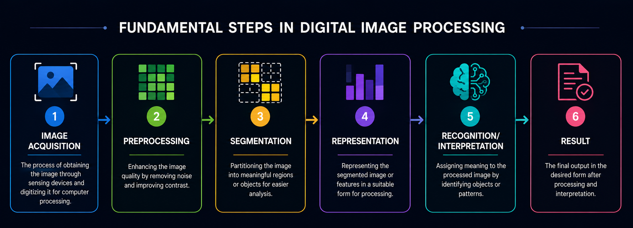
Steps in Digital Image Processing:

🖼️ Fundamental Steps in DIP

Types of Digital Images:

Type	Description
Binary Image	Only 2 intensity values: 0 (black) and 1 (white)
Grayscale Image	Intensity values from 0 to 255 (8-bit) — shades of gray
Color Image	3 channels — Red, Green, Blue (RGB), each 0-255

💡 Exam Tip: Remember f(x,y) notation — x,y are the PIXEL COORDINATES (position), and f is the INTENSITY (gray level/brightness) at that position. This distinction (position vs value) is fundamental and comes up throughout the unit.

2. Sampling and Quantization

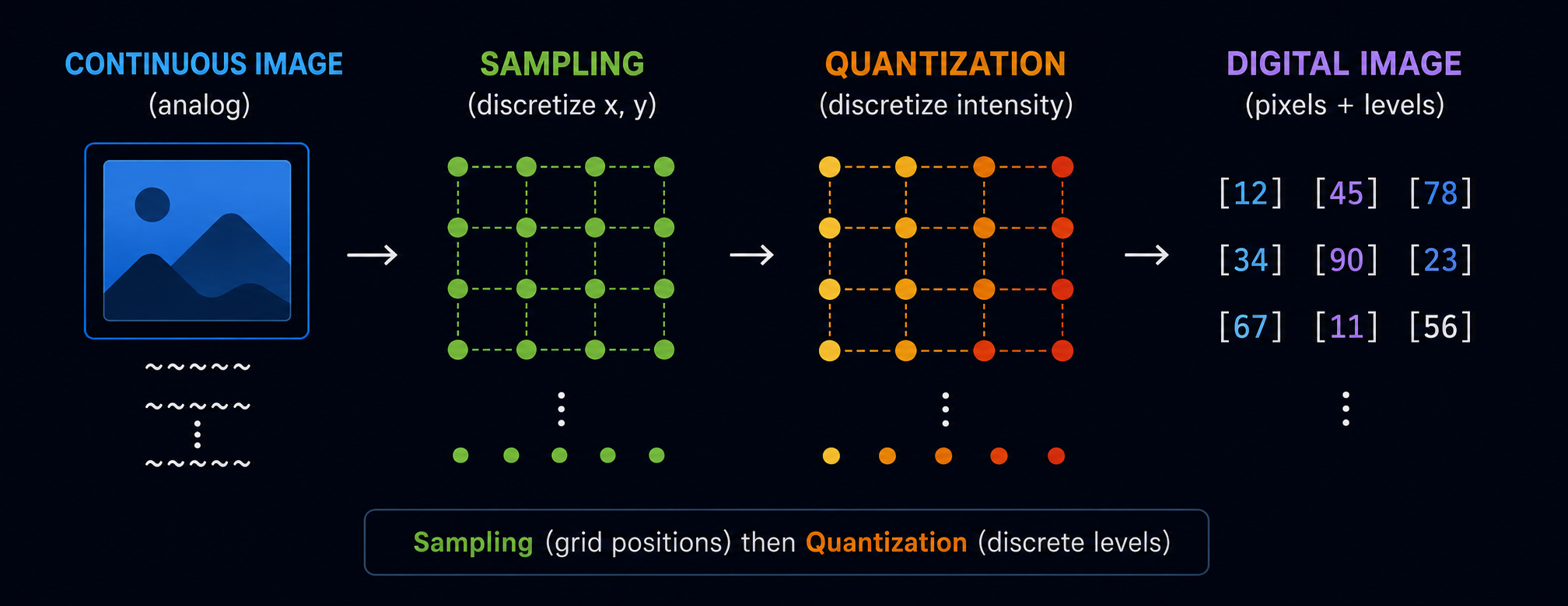
📖 Sampling: Digitizing the SPATIAL coordinates (x,y) — converting a continuous image into a grid of discrete pixel positions.

📖 Quantization: Digitizing the AMPLITUDE (intensity) values — converting continuous brightness into a finite number of discrete gray levels.

Sampling Grid Positions Then Quantization Discrete Levels

📊 Sampling and Quantization

Storage Size Formula:
Number of bits required = M × N × k
where M×N = image dimensions (rows × columns), k = bits per pixel, and L = 2^k = number of gray levels

💡 Worked Example: Find the storage size (in bits and bytes) for a 256×256 image with 256 gray levels.

M = 256, N = 256
L = 256 = 2⁸ → k = 8 bits/pixel
Total bits = 256 × 256 × 8 = 524,288 bits
Total bytes = 524,288 / 8 = 65,536 bytes = 64 KB

💡 Worked Example — Reverse Calculation: How many gray levels (L) are needed if 6 bits are used per pixel?

L = 2^k = 2⁶ = 64 gray levels (intensity values from 0 to 63)

Concept	Effect of INCREASING it
Sampling Rate ↑ (more pixels)	Better spatial resolution — finer detail, sharper image
Quantization Levels ↑ (more gray levels)	Better tonal/intensity resolution — smoother gradients, less "banding"

⚠️ Low Sampling → Checkerboard/Blocky effect.
⚠️ Low Quantization → False Contouring (visible bands/steps in what should be a smooth gradient, e.g. reducing 256 levels down to just 4-8 levels).

💡 Exam Tip: "Bits needed" numericals are extremely common — always identify M, N, and L (or k) from the question first, then apply Bits = M×N×k directly. Don't forget to convert bits→bytes (÷8) if the question asks for storage in bytes/KB/MB.

3. Relationships Between Pixels

A. Neighbors of a Pixel:

Type	Notation	Pixels Included
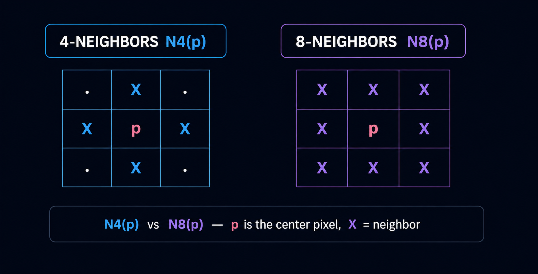
4-Neighbors	N₄(p)	Up, Down, Left, Right (horizontal + vertical only)
Diagonal Neighbors	N_D(p)	The 4 diagonal pixels
8-Neighbors	N₈(p)	N₄(p) + N_D(p) combined (all 8 surrounding pixels)

🧩 N4(p) vs N8(p) Pixel Neighbors

B. Adjacency & Connectivity:

Type	Rule
4-Adjacency	Two pixels are adjacent if they're in each other's N₄ set AND have similar intensity values
8-Adjacency	Two pixels are adjacent if they're in each other's N₈ set AND have similar intensity values
m-Adjacency (mixed)	Solves ambiguity in 8-adjacency — used when diagonal AND direct adjacency conflict

C. Distance Measures:

For two pixels p(x,y) and q(s,t):

Euclidean Distance: D_e = √[(x−s)² + (y−t)²]
City-Block (Manhattan) Distance: D₄ = |x−s| + |y−t|
Chessboard Distance: D₈ = max(|x−s|, |y−t|)

💡 Worked Example: Find all 3 distances between p(2,3) and q(6,7).

|x−s| = |2−6| = 4, |y−t| = |3−7| = 4

D_e = √(4² + 4²) = √32 = 5.66
D₄ (City-Block) = 4 + 4 = 8
D₈ (Chessboard) = max(4, 4) = 4

💡 Exam Tip: D₈ (Chessboard) ≤ D_e (Euclidean) ≤ D₄ (City-Block) — always holds true. Memorize this ordering to sanity-check your numerical answers.

4. Image Transforms — 2D FFT (Discrete Fourier Transform)

📖 Why Transform an Image? Transforms convert an image from the SPATIAL domain (pixel values) into another domain (like FREQUENCY) where certain operations — filtering, compression, feature extraction — become easier or more efficient.

📖 2D-DFT: Decomposes an image into a sum of sinusoidal (sine/cosine) components at different frequencies, revealing how much of each frequency is present.

2D Discrete Fourier Transform:
F(u,v) = (1/MN) ΣΣ f(x,y)·e^(−j2π(ux/M + vy/N))
for x=0..M−1, y=0..N−1

Inverse 2D-DFT:
f(x,y) = ΣΣ F(u,v)·e^(+j2π(ux/M + vy/N))

Property	Description
Linearity	DFT of a sum = sum of individual DFTs
Translation	Shifting an image in spatial domain only changes the PHASE of its Fourier Transform, not the magnitude
Periodicity	F(u,v) is periodic — repeats with period M (or N)
Symmetry (Conjugate)	For real input images, F(−u,−v) = F*(u,v) (complex conjugate)
Rotation	Rotating the image rotates its Fourier Transform by the SAME angle
Scaling	Scaling the image inversely scales its Fourier Transform
Separability	2D-DFT can be computed as two successive 1D-DFTs (rows then columns) — massively speeds up computation

✅ Why Separability Matters: Computing a 2D-DFT directly is expensive; using separability (rows first, then columns) reduces the computational complexity dramatically — this is the core idea behind the Fast Fourier Transform (FFT) algorithm.

💡 Exam Tip: F(0,0) is called the "DC component" — it equals the AVERAGE intensity of the entire image (sum of all pixel values divided by MN). This is a favorite conceptual/numerical question.

5. Walsh Transform & Hadamard Transform

📖 Why these transforms? Unlike Fourier Transform (which uses sine/cosine — needs complex/floating-point math), Walsh and Hadamard transforms use ONLY +1 and −1 values — making them extremely fast to compute (just additions/subtractions, no multiplication).

A. Walsh Transform:

Based on Walsh functions — a set of orthogonal, rectangular waveforms taking only values +1 and −1. The Walsh Transform kernel is built from bit-reversed binary representations of the indices.

B. Hadamard Transform:

Very similar to Walsh — uses a Hadamard MATRIX (also entries of only +1/−1), constructed RECURSIVELY.

Hadamard Matrix Construction (recursive):
H₁ = [1]
H₂ₙ = [ Hₙ Hₙ ; Hₙ −Hₙ ] (block matrix form)

💡 Worked Example — H₂ (2×2 Hadamard Matrix):
H₂ = [ 1 1 ; 1 −1 ]

H₄ (4×4), built from H₂:
H₄ = [ H₂ H₂ ; H₂ −H₂ ] =
[ 1 1 1 1 ]
[ 1 −1 1 −1 ]
[ 1 1 −1 −1 ]
[ 1 −1 −1 1 ]

Feature	Walsh	Hadamard
Values used	+1, −1	+1, −1
Ordering of basis functions	Sequency order (number of sign changes)	Natural/recursive order
Matrix construction	Bit-reversal based	Simple recursive doubling
Computation speed	Very fast (no multiplication)	Very fast (no multiplication)

💡 Exam Tip: The KEY advantage of both transforms over DFT: since the transform matrix contains ONLY +1 and −1, computing the transform requires only ADDITION and SUBTRACTION — no multiplication needed at all, making them much faster in hardware.

6. Discrete Cosine Transform (DCT)

📖 DCT: Represents an image as a sum of COSINE functions oscillating at different frequencies — similar to DFT, but uses only REAL (cosine) values, no imaginary/complex numbers.

1D-DCT Formula:
C(u) = α(u) Σ f(x)·cos[ π(2x+1)u / 2N ] for x=0..N−1

where α(0) = √(1/N), and α(u) = √(2/N) for u≠0

✅ Why DCT is used in JPEG Compression:
1. Energy Compaction: Most of an image's important visual information gets concentrated into just a FEW low-frequency DCT coefficients — high-frequency coefficients (fine detail/noise) can be discarded with minimal visible quality loss.
2. Real-valued output (unlike DFT's complex numbers) — simpler to store and process.
3. No artificial periodicity/discontinuity issues that DFT can introduce at block boundaries.

Feature	DFT	DCT
Output type	Complex numbers	Real numbers only
Basis functions	Sine + Cosine	Cosine only
Energy compaction	Good	Better (more concentrated)
Common use	General frequency analysis	JPEG, image/video compression

💡 Exam Tip: "Why is DCT preferred over DFT for image compression?" is a classic conceptual question — the answer is always ENERGY COMPACTION (concentrating information into fewer coefficients) + REAL-valued output (simpler than DFT's complex numbers).

7. Haar Transform & Slant Transform

A. Haar Transform:

📖 Haar Transform: Based on Haar functions — the simplest form of WAVELET transform, made of rectangular pulse pairs. Unlike Fourier-based transforms, Haar captures BOTH frequency AND spatial location information simultaneously.

✅ Key Advantage: Excellent for detecting sharp changes/edges and localizing WHERE in the image a particular frequency component occurs — Fourier-based transforms only tell you WHAT frequencies exist, not WHERE.

B. Slant Transform:

📖 Slant Transform: Contains basis vectors that include "slant" (linearly/ramp-varying) functions — specifically designed to efficiently represent gradually changing brightness (gradients/ramps) common in real images (e.g. shading, gradual lighting changes).

Transform	Best For	Key Property
Haar	Edge detection, sharp transitions	Captures location + frequency (wavelet-based)
Slant	Smooth gradients/ramps	Includes ramp-like basis vectors for efficient gradient representation

💡 Exam Tip: Haar Transform is often introduced as the EARLIEST/simplest wavelet — a common question is "Haar Transform is a special case of which broader class of transforms?" → Answer: Wavelet Transforms.

8. Hotelling Transform (Karhunen-Loève Transform)

📖 Hotelling Transform: Also called Karhunen-Loève Transform (KLT) or Principal Component Analysis (PCA) in general statistics — transforms data using the EIGENVECTORS of the data's covariance matrix, so the transformed data has NO correlation between its components.

Basic Steps:
1. Compute the MEAN vector of the input data
2. Compute the COVARIANCE matrix of the data
3. Find the EIGENVALUES and EIGENVECTORS of the covariance matrix
4. Arrange eigenvectors in DECREASING order of their eigenvalues — these become the new transform basis
5. Project the original data onto these eigenvectors

✅ Why it's "Optimal": Unlike DFT/DCT/Walsh/Hadamard (which use FIXED, pre-determined basis functions regardless of the input), the Hotelling Transform's basis is DATA-DEPENDENT — computed directly from the statistics of the specific image/dataset. This makes it mathematically OPTIMAL for compacting energy into the fewest possible coefficients (best possible compression, in theory).

❌ Practical Drawback: Since the basis vectors depend on the input data, they must be RECOMPUTED for every new image/dataset (unlike DCT which uses the same fixed cosine basis every time) — this makes Hotelling Transform computationally EXPENSIVE and impractical for real-time/general-purpose compression, despite being theoretically optimal.

💡 Exam Tip: "Why isn't the Hotelling Transform used in practice as widely as DCT, despite being optimal?" → Because its basis functions are DATA-DEPENDENT (must be recalculated every time), unlike DCT's FIXED basis — a classic theory-vs-practicality trade-off question.

✨ Chapter 2 — Image Enhancement

✨ CHAPTER 2 — IMAGE ENHANCEMENT MIND MAP

Point Operations → Negative(s=L-1-r), Log(expand dark), Power-Law/Gamma(γ<1 brighten, γ>1 darken)

Histogram Equalization → s_k=(L-1)×CDF, spreads histogram for better contrast

Gray Level Transform → Contrast Stretching(linear) vs Slicing/Bit-plane(non-linear)

Median Filter → sort neighborhood, pick middle value; great for salt-pepper noise

Spatial High-Pass → Laplacian, Unsharp Masking(k=1), High-Boost(k>1)

Frequency Filtering → G(u,v)=H(u,v)×F(u,v), Convolution Theorem

Low-Pass → Ideal(ringing) → Butterworth(adjustable) → Gaussian(smooth, no ringing)

High-Pass → H_HP = 1 - H_LP (derived directly from low-pass)

1. Introduction to Spatial Domain Enhancement

📖 Image Enhancement: The process of adjusting an image to make it more suitable for a specific application — improving visual quality or highlighting particular features (unlike restoration, enhancement doesn't need a mathematical "ground truth" model of degradation).

📖 Spatial Domain: Techniques that operate DIRECTLY on the pixel values of the image itself — as opposed to Frequency Domain, which first transforms the image (e.g. via DFT) before processing.

General Spatial Domain Operation:
g(x,y) = T[f(x,y)]
where f = input image, g = output (processed) image, T = some operator/transformation applied to f

Categories of Spatial Domain Operations:

Category	How T Operates	Example
Point Operations	T depends ONLY on the value of f at a SINGLE pixel (x,y)	Image Negative, Log Transform, Power-Law
Neighborhood (Mask/Filter) Operations	T depends on f in a small NEIGHBORHOOD around (x,y)	Smoothing, Sharpening, Median Filter
Geometric/Global Operations	T depends on the ENTIRE image or geometric transformation rules	Rotation, Scaling

💡 Exam Tip: Point operations are the SIMPLEST — output depends only on that ONE pixel's input value, with no regard for neighboring pixels. This is the key distinguishing feature examiners test for "define point operation" questions.

2. Point Operations — Negative, Log & Power-Law Transform

A. Image Negative:

s = L − 1 − r
r = input intensity, s = output intensity, L = number of gray levels

💡 Worked Example: For an 8-bit image (L=256), find the negative of a pixel with intensity r=60.
s = 256 − 1 − 60 = 195

B. Log Transformation:

s = c · log(1 + r)
c = scaling constant, usually c = (L−1)/log(1+r_max)

✅ Use: EXPANDS dark pixel values while COMPRESSING bright ones — useful for displaying images with a very large dynamic range (e.g. Fourier spectrum images, which have a few very bright pixels and lots of dark ones).

C. Power-Law (Gamma) Transformation:

s = c · r^γ
c and γ (gamma) are positive constants

💡 Worked Example: Given c=1, apply Power-Law with γ=0.5 (square-root, brightens image) to r=0.36 (normalized intensity 0-1 scale).
s = 1 × (0.36)^0.5 = 0.6 (brighter than input)

γ value	Effect
γ < 1	Brightens the image (expands dark tones)
γ = 1	No change (identity — output = input)
γ > 1	Darkens the image (expands bright tones)

💡 Exam Tip: Power-Law/Gamma correction is used to compensate for the non-linear response of display devices (monitors, TVs, cameras) — "gamma correction" is the direct real-world application examiners like to ask about.

3. Histogram Manipulation — Histogram Equalization

📖 Histogram: A plot showing the FREQUENCY (count) of each intensity/gray level occurring in an image.

📖 Histogram Equalization: A technique that redistributes intensity values so the output histogram is as UNIFORM/spread-out as possible — improving contrast in images that are too dark, too bright, or low-contrast.

Equalization Formula:
s_k = (L−1) · Σ(n_j / n) for j = 0 to k
n_j = number of pixels with intensity j, n = total pixels, L = number of gray levels

Worked Example — 3-bit image (L=8), 64 total pixels:

r_k	n_k (count)	PDF (n_k/n)	CDF (cumulative)	s_k = 7×CDF (rounded)
0	8	0.125	0.125	1
1	10	0.156	0.281	2
2	12	0.188	0.469	3
3	14	0.219	0.688	5
4	10	0.156	0.844	6
5	6	0.094	0.938	7
6	3	0.047	0.984	7
7	1	0.016	1.000	7

💡 How to Read This Table (step-by-step method):
1. Count occurrences n_k of each intensity level (given/observed from the image)
2. Compute PDF = n_k / total pixels (n)
3. Compute CDF = running cumulative SUM of PDF values so far
4. New intensity s_k = (L−1) × CDF, then ROUND to the nearest integer
5. Remap every pixel of old intensity r_k to the new intensity s_k

✅ Result: Original 8 intensity levels get remapped/compressed into effectively 6 distinct output levels (1,2,3,5,6,7) — but the histogram of the NEW image is much more spread out/uniform than the original, improving overall contrast.

💡 Exam Tip: Histogram equalization questions ALWAYS want the full table (r_k, n_k, PDF, CDF, s_k) shown step by step — never skip straight to the final remapped values. Also note: some very close CDF values can round to the SAME s_k, which is why the output may end up with FEWER distinct gray levels than the input.

4. Linear and Non-Linear Gray Level Transformations

📖 Gray Level Transformation: A function that maps each input intensity r to an output intensity s, used to enhance contrast or highlight specific intensity ranges.

A. Linear Transformation — Contrast Stretching:

Contrast Stretching:
s = [(s₂−s₁)/(r₂−r₁)] × (r−r₁) + s₁
Stretches the range [r₁,r₂] of input intensities to the FULL range [s₁,s₂] of output intensities

💡 Worked Example: An image has intensities in the range [50,150]. Stretch this to the full [0,255] range. Find the output for r=100.

s = [(255−0)/(150−50)] × (100−50) + 0
s = (255/100) × 50 = 2.55 × 50 = 127.5 ≈ 128

B. Non-Linear Transformation — Gray Level Slicing:

Gray Level Slicing: Highlights a SPECIFIC range of intensities (e.g. to emphasize certain features) while either:
(a) setting all other intensities to a LOW constant value, or
(b) preserving all other intensities as their ORIGINAL background values

C. Non-Linear — Bit-Plane Slicing:

📖 Bit-Plane Slicing: An 8-bit image can be viewed as 8 separate 1-bit "bit planes" (from the MSB/bit-7 down to the LSB/bit-0). Higher-order bit planes contain most of the visually significant data; lower-order planes contain fine detail/noise.

💡 Exam Tip: Contrast stretching is LINEAR (a straight-line mapping equation); Gray-level slicing and Bit-plane slicing are NON-LINEAR (they involve conditional/piecewise rules, not one continuous straight line). This linear-vs-nonlinear classification is a common 2-mark question.

5. Neighborhood Operations & Median Filter

📖 Neighborhood (Mask) Operation: The output at pixel (x,y) depends on the values of f in a small NEIGHBORHOOD (e.g. 3×3 window) surrounding (x,y), not just f(x,y) alone.

📖 Median Filter: A non-linear neighborhood filter that replaces each pixel's value with the MEDIAN (middle value when sorted) of the intensities in its neighborhood — excellent for removing "salt-and-pepper" (impulse) noise while preserving edges.

Worked Example — 3×3 Median Filter:

Original 3×3 neighborhood (center pixel has noise = 255): 10 12 11 13 255 14 ← center pixel corrupted (salt noise) 12 11 13

Fig: 3×3 Neighborhood with Noisy Center Pixel

Step 1: Collect all 9 values: 10, 12, 11, 13, 255, 14, 12, 11, 13 Step 2: Sort them in ascending order: 10, 11, 11, 12, 12, 13, 13, 14, 255 Step 3: Find the MIDDLE (5th) value: 10, 11, 11, 12, [12], 13, 13, 14, 255 ↑ This is the MEDIAN Step 4: Replace center pixel with median = 12

✅ Result: The noisy pixel (255) is replaced by 12 — matching its neighbors closely, effectively removing the noise spike WITHOUT blurring the surrounding edges (unlike a simple averaging/mean filter, which would still be dragged toward 255).

Feature	Mean (Averaging) Filter	Median Filter
Type	Linear	Non-linear
Best for	Gaussian noise	Salt-and-pepper (impulse) noise
Edge Preservation	Blurs edges	Preserves edges well
Effect of extreme outlier	Drags average toward outlier	Outlier gets discarded (not the median)

💡 Exam Tip: Median filter numericals always follow the SAME 4 steps — collect neighborhood values, sort them, pick the middle one (median), replace the center pixel. For a 3×3 window (9 values), the median is always the 5th value after sorting.

6. Spatial Domain High-Pass Filtering

📖 High-Pass Filtering: Enhances/sharpens fine details, edges, and rapid intensity changes in an image, while SUPPRESSING slowly-varying (smooth) regions — the opposite goal of low-pass (smoothing) filters.

Laplacian Filter (2nd derivative-based):

Laplacian Mask (common 3×3 kernel):
[ 0 −1 0 ]
[−1 4 −1 ]
[ 0 −1 0 ]

Sharpening using Laplacian:
g(x,y) = f(x,y) + c·∇²f(x,y)
(original image PLUS the Laplacian result, to add back the enhanced edges — c is typically +1 or −1 depending on the mask's center sign convention)

Unsharp Masking & High-Boost Filtering:

📖 Unsharp Masking: Subtract a BLURRED (low-pass filtered) version of the image from the original — the difference highlights the fine edges/detail, which is then added back to sharpen.

Unsharp Masking: g_mask(x,y) = f(x,y) − f_blurred(x,y)
g(x,y) = f(x,y) + k·g_mask(x,y) (k=1 for standard unsharp masking)

High-Boost Filtering: Same formula but with k > 1 — amplifies the sharpening effect further.

💡 Exam Tip: High-Boost Filtering is just Unsharp Masking with an amplification factor k > 1 — when k=1 they're identical; the ONLY difference is the strength of the sharpening applied.

7. Frequency Domain Filtering — Basics

📖 Frequency Domain Filtering: Instead of directly manipulating pixels, the image is first transformed (via DFT) into the frequency domain, MULTIPLIED by a filter function H(u,v), then transformed BACK to the spatial domain using the Inverse DFT.

f(x,y) --DFT--> F(u,v) --×H(u,v)--> G(u,v) --Inverse DFT--> g(x,y) (input) (frequency) (filtered) (output)

Fig: General Frequency Domain Filtering Process

Core Relationship (Convolution Theorem):
G(u,v) = H(u,v) · F(u,v)
Multiplication in FREQUENCY domain = Convolution in SPATIAL domain

A. Obtaining Frequency Domain Filters from Spatial Filters:

Take an existing spatial-domain filter mask (like the Laplacian kernel), and compute its DFT — this gives the equivalent frequency-domain filter H(u,v) that would produce the SAME result if used in the frequency domain.

B. Generating Filters Directly in the Frequency Domain:

Instead of converting a spatial filter, DESIGN the filter H(u,v) directly based on desired frequency response — e.g. deciding exactly which frequency ranges to pass or block (this is how Ideal/Butterworth/Gaussian filters, covered next, are typically specified).

💡 Exam Tip: The Convolution Theorem is the SINGLE most important formula in this section — it's what makes frequency-domain filtering possible at all (multiplication is computationally simpler than convolution for large images/masks).

8. Low-Pass (Smoothing) Filters in Frequency Domain

📖 Low-Pass Filter (LPF): ALLOWS low frequencies (smooth, slowly-varying regions) to pass through, while BLOCKING/attenuating high frequencies (edges, noise, fine detail) — result: a blurred/smoothed image.

A. Ideal Low-Pass Filter (ILPF):

H(u,v) = 1, if D(u,v) ≤ D₀
H(u,v) = 0, if D(u,v) > D₀

D(u,v) = distance from point (u,v) to the center of the frequency rectangle, D₀ = cutoff frequency

❌ Problem — Ringing Effect: The SHARP cutoff (sudden jump from 1 to 0) causes visible "ringing" artifacts (oscillating rings) around edges in the output image.

B. Butterworth Low-Pass Filter (BLPF):

H(u,v) = 1 / [1 + (D(u,v)/D₀)^(2n)]
n = order/degree of the filter

✅ Advantage over ILPF: SMOOTH transition (not a sudden cutoff) — significantly reduces ringing artifacts. Higher order "n" makes the transition sharper (behaves more like ILPF); lower "n" gives a gentler transition.

C. Gaussian Low-Pass Filter (GLPF):

H(u,v) = e^(−D(u,v)²/2D₀²)

✅ Advantage: COMPLETELY smooth transition (Gaussian curve) — produces NO ringing artifacts at all, though it may smooth/blur slightly more than an equivalent Butterworth filter.

Filter	Transition	Ringing?
Ideal (ILPF)	Sharp/sudden cutoff	Severe ringing
Butterworth (BLPF)	Smooth, adjustable via order n	Mild ringing (less as n decreases)
Gaussian (GLPF)	Completely smooth	No ringing

💡 Exam Tip: "Why does Gaussian filter avoid ringing while Ideal filter doesn't?" → A sharp cutoff in the frequency domain corresponds to a "sinc"-shaped ripple pattern in the spatial domain (Gibbs phenomenon) — smooth transitions (Gaussian, Butterworth) avoid this abrupt discontinuity.

9. High-Pass (Sharpening) Filters in Frequency Domain

📖 High-Pass Filter (HPF): The OPPOSITE of low-pass — BLOCKS low frequencies (smooth regions) and ALLOWS high frequencies (edges, fine detail) to pass through, sharpening the image.

Key Relationship: H_HP(u,v) = 1 − H_LP(u,v)
Every High-Pass filter can be derived by simply SUBTRACTING the corresponding Low-Pass filter's response from 1.

Filter	Formula (derived from LPF)
Ideal HPF (IHPF)	H=0 if D≤D₀, H=1 if D>D₀ (exact reverse of ILPF)
Butterworth HPF (BHPF)	H(u,v) = 1 / [1 + (D₀/D(u,v))^(2n)]
Gaussian HPF (GHPF)	H(u,v) = 1 − e^(−D(u,v)²/2D₀²)

💡 Same Trade-offs as Low-Pass (mirrored):
Ideal HPF → sharp cutoff → ringing artifacts.
Butterworth HPF → adjustable smoothness via order n → mild/reduced ringing.
Gaussian HPF → smoothest transition → no ringing, cleanest sharpening.

High-Frequency Emphasis Filtering:

H_emphasis(u,v) = a + b·H_HP(u,v) where a≥0, b>a
(adds back a fraction "a" of the original low-frequency content, so the image isn't left looking completely flat/gray after high-pass filtering)

💡 Exam Tip: Since H_HP = 1 − H_LP, once you know any Low-Pass filter formula, you can derive its High-Pass counterpart instantly — examiners often test this relationship directly ("derive the Butterworth HPF from the BLPF formula").

📚 Self-Study Topic

Self-Study Topic — Concepts of Digital Signal Processing 📚 Extra Reading

📌 Note: Listed as Self-Study in the syllabus — good foundational background for understanding why image processing techniques (sampling, transforms, filtering) work the way they do. A digital image is essentially a 2D SIGNAL.

📖 Digital Signal Processing (DSP): The field of analyzing, modifying, and synthesizing signals (audio, image, sensor data) represented as discrete/digital sequences of numbers, using mathematical operations.

DSP Concept	Connection to Image Processing
Sampling Theorem (Nyquist)	Determines minimum sampling rate needed to avoid aliasing — same principle applies to spatial sampling of images
Convolution	Core operation behind spatial filtering (masks/kernels) in image processing
Fourier Transform	1D signal FT extends directly to 2D image FT — same math, one more dimension
Filtering (Low-pass/High-pass)	Same low-pass = smoothing, high-pass = sharpening concepts as in audio signal processing
Quantization	Same amplitude-discretization concept as digitizing analog audio signals

💡 Key Insight: A digital IMAGE is just a 2D extension of a 1D digital SIGNAL — almost every technique covered in this unit (sampling, quantization, transforms, filtering) is a direct application of standard 1D Digital Signal Processing theory, extended into two dimensions (x and y).

⚡ Ready for Exam? Sab padh liya? Ab Quick Revision karo — formulas, numericals aur key points ek jagah! Quick Revision Karo →

⚡ Quick Revision — Last Minute Exam Prep!

📌 How to Use: Read this 5-10 minutes before exam. Contains all important points in condensed form. Focus on tables, comparisons, and key formulas!

🖼️ Chapter 1 — Digital Image Fundamentals

📖 f(x,y): x,y = position (spatial coords), f = intensity/gray level at that position.

SAMPLING & QUANTIZATION:
Bits required = M × N × k (k=bits/pixel, L=2^k gray levels)

Quick Recall: 256×256 image, 256 levels (k=8) → 256×256×8 = 524,288 bits = 64 KB

🔑 Distance Measures — p(x,y), q(s,t):

Euclidean: D_e = √[(x−s)²+(y−t)²]
City-Block: D₄ = |x−s|+|y−t|
Chessboard: D₈ = max(|x−s|,|y−t|)

Order: D₈ ≤ D_e ≤ D₄

✅ Transforms Quick Recall:
2D-DFT → complex, separable, F(0,0)=DC=average intensity
Walsh/Hadamard → only +1/−1, no multiplication needed
DCT → real-valued, energy compaction, used in JPEG
Haar → wavelet, captures location+frequency
Slant → ramp/gradient basis functions
Hotelling/KLT → eigenvector-based, optimal but data-dependent (expensive)

Topic	Key Fact	Trick
Sampling vs Quantization	Position vs Intensity digitization	Low sampling→blocky; Low quantization→false contouring
N4 vs N8 neighbors	4 direct vs 4 direct+4 diagonal	N8 = N4 + N_Diagonal
DCT vs DFT	Real vs Complex output	DCT better energy compaction
Hotelling Transform	Data-dependent basis	Optimal but must recompute every time

✨ Chapter 2 — Image Enhancement

📖 Point Operations — Quick Formulas:
Negative: s = L−1−r
Log: s = c·log(1+r) — expands dark, compresses bright
Power-Law: s = c·r^γ — γ<1 brightens, γ>1 darkens

🔑 Histogram Equalization — Steps:
1. Count n_k per level → 2. PDF = n_k/n → 3. CDF = cumulative PDF → 4. s_k = (L−1)×CDF, round

Formula: s_k = (L−1)·Σ(n_j/n)

MEDIAN FILTER — Quick Recall:
Collect 3×3 neighborhood (9 values) → Sort → Pick 5th (middle) value → Replace center
Best for: salt-and-pepper noise. Preserves edges (unlike mean filter).

✅ Frequency Domain Filters:
G(u,v) = H(u,v)×F(u,v) (Convolution Theorem)
Ideal → sharp cutoff, ringing
Butterworth → adjustable (order n), mild ringing
Gaussian → smooth, no ringing

H_HP = 1 − H_LP (derive High-Pass from Low-Pass directly)

Topic	Key Fact	Trick
Contrast Stretching	Linear mapping equation	vs Gray-slicing/Bit-plane (non-linear)
Median Filter	Non-linear, sorts + picks middle	3×3 window → 5th value after sort
Unsharp Masking	k=1	High-Boost = same formula, k>1
Ideal Filter	Sharp cutoff	Causes ringing (Gibbs phenomenon)
Gaussian Filter	Smooth transition	No ringing at all

⚠️ Common Exam Mistakes

❌ Confusing Sampling (position digitization) with Quantization (intensity digitization)
❌ Forgetting to convert bits→bytes (÷8) when a storage numerical asks for KB/MB
❌ Mixing up City-Block (sum of differences) with Chessboard (max of differences) distance
❌ Confusing DFT (complex output) with DCT (real-valued output) — DCT is preferred for compression due to energy compaction
❌ In Histogram Equalization, forgetting to ROUND s_k to the nearest integer, or skipping the PDF/CDF table steps
❌ Applying Mean filter logic to a Median filter question (median = sort + pick middle, NOT an average)
❌ Forgetting H_HP = 1 − H_LP — deriving a High-Pass filter formula from scratch instead of this direct relationship
❌ Saying Ideal filters are "better" because of the name — they actually cause the WORST ringing artifacts

✅ Pre-Exam Checklist

☑ f(x,y) notation — position vs intensity
☑ Sampling/Quantization + storage size numericals (M×N×k)
☑ Pixel neighbors (N4/N8) + distance measures (Euclidean/City-Block/Chessboard) numericals
☑ 2D-FFT properties (especially separability, DC component)
☑ Walsh/Hadamard — matrix construction, +1/−1 property
☑ DCT — formula, why preferred over DFT for compression
☑ Haar vs Slant transform differences
☑ Hotelling/KLT — steps, optimal but data-dependent trade-off
☑ Point operations — Negative/Log/Power-Law formulas + numericals
☑ Histogram Equalization — full worked table method
☑ Contrast Stretching numerical + linear vs non-linear classification
☑ Median filter — full worked 3×3 example
☑ Laplacian/Unsharp Masking/High-Boost formulas
☑ Convolution theorem — G(u,v)=H(u,v)×F(u,v)
☑ Ideal/Butterworth/Gaussian Low-Pass — formulas + ringing trade-offs
☑ High-Pass filters derived from Low-Pass (1−H_LP relationship)

🎯 Exam Strategy

2 Mark Questions:
• Direct definition/formula + 1 small example. Time: 3-4 minutes.
• "Differentiate" → always draw a 2-column table.

5 Mark Questions:
• Numericals (sampling/quantization, distance measures, histogram equalization, median filter) — show EVERY step in a table/sequence, don't skip to the final answer.
• Filter comparison questions — always mention the ringing artifact trade-off (Ideal vs Butterworth vs Gaussian).
• Time: 7-8 minutes per question.

Marks-saving tip:
Even if a full numerical isn't finished, writing the correct formula and correctly identifying the given values (M,N,k or r_k,n_k) earns partial marks!

🌟 All the Best!
DIP Unit 1 is numerical-heavy — sampling/quantization, distance measures, histogram equalization, aur median filter practice karo by hand, step by step. Formulas aur filter trade-offs yaad karo, aur tu ready hai! 💪🖼️

📄 Previous Year Questions

Previous Year Question Paper Not Available Yet

Previous year question papers for this unit are not available yet. If you have the question paper, please share it through the contact page so it can be added for other students.

Share Question Paper

📚 Chapters

🖼️ Digital Image Processing

1. Digital Image Fundamentals

2. Sampling and Quantization

3. Relationships Between Pixels

4. Image Transforms — 2D FFT (Discrete Fourier Transform)

5. Walsh Transform & Hadamard Transform

6. Discrete Cosine Transform (DCT)

7. Haar Transform & Slant Transform

8. Hotelling Transform (Karhunen-Loève Transform)

1. Introduction to Spatial Domain Enhancement

2. Point Operations — Negative, Log & Power-Law Transform

3. Histogram Manipulation — Histogram Equalization

4. Linear and Non-Linear Gray Level Transformations

5. Neighborhood Operations & Median Filter

6. Spatial Domain High-Pass Filtering

7. Frequency Domain Filtering — Basics

8. Low-Pass (Smoothing) Filters in Frequency Domain

9. High-Pass (Sharpening) Filters in Frequency Domain

Self-Study Topic — Concepts of Digital Signal Processing 📚 Extra Reading

🖼️ Chapter 1 — Digital Image Fundamentals

✨ Chapter 2 — Image Enhancement

⚠️ Common Exam Mistakes

✅ Pre-Exam Checklist

🎯 Exam Strategy

Previous Year Question Paper Not Available Yet